Overview

What is Simulation-Based Inference?

Traditional LHC analyses compress high-dimensional collision data into summary observables before performing statistical inference. This dimensionality reduction is convenient, since it allows efficient histogram-based density estimation, but it can discard information that is sensitive to the parameters of interest.

In SBI we approximate the likelihood ratio directly from the full feature space using neural network surrogates. The result is a statistical model that can extract more information from the same data.

In practice, a pure machine-learning likelihood is not scalable: LHC analyses must account for dozens of systematic uncertainties (detector calibrations, theory variations, luminosity, etc.) and combine signal-enriched regions with data-driven control regions. This toolkit bridges the gap between phenominlogical proof-of-concepts and real measurements at the LHC by embedding neural density-ratio estimates inside a HistFactory-style statistical model, also referred to as a semi-parametric SBI model, so that the full LHC-style statistical model can be built using SBI and so both unbinned SBI regions and traditional binned template regions contribute to a single profiled-likelihood fit. This is done via easy-to-use APIs for the various stages in the analysis as well as providing an end-to-end workflow orchestration pipeline steered via human-readable configuration files.

The toolkit is designed to be modular and extensible. The built-in PyTorch Lightning modules (density-ratio estimation via binary classification, multi-class region classification) cover the most common use cases, but the training utilities, ONNX export pipeline, and statistical model infrastructure are model-agnostic — users can plug in alternative architectures (e.g. normalising flows for direct density estimation, graph neural networks, transformers) without significantly modifying the downstream fitting machinery.

For more details on the method, see arXiv:2412.01600. The first measurement using this technique — off-shell Higgs boson production in the \(H\to ZZ \to 4\ell\) channel with ATLAS — is described in arXiv:2412.01548.

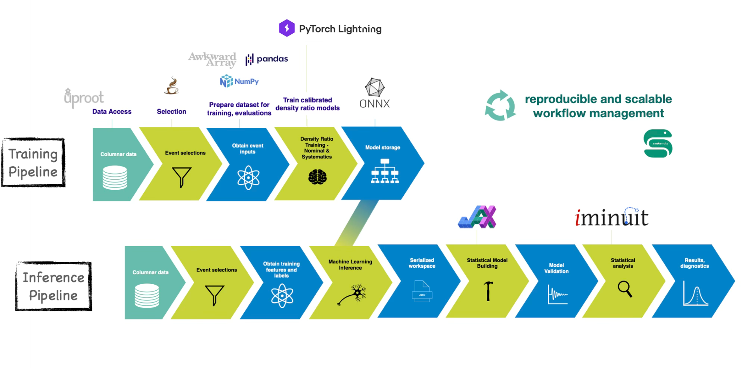
High-level overview of the SBI workflow and the various stages.

How the pieces fit together

The analysis pipeline has four stages:

1. Data preparation — Load ROOT ntuples, apply preselection, split into analysis regions (binned control regions, unbinned signal region).

2. Training — For each physics process (basis point), train an ensemble of density-ratio neural networks that learn \(r(x) = p_{\text{process}}(x) / p_{\text{reference}}(x)\). Systematic variations get their own ensemble models.

3. Evaluation — Run the trained networks on the full Asimov or real dataset to produce per-event density-ratio arrays. These arrays, together with the binned histograms and systematic variation templates, are assembled into a serialized workspace — a JSON-like dictionary that fully specifies the statistical model.

4. Fitting — The workspace is passed to sbi_parametric_model, which compiles a JAX-based NLL function. This is minimised by inference to extract the best-fit parameters and profile-likelihood scans. We will soon add the functionality to run Neyman Construction.